はじめに #
PyomoというPythonライブラリを使って線形計画問題を解く方法をまとめた。 本記事ではPyomoの導入方法と、問題の記述方法について示す。
PyomoはPythonで書かれた最適化モデリングツールである。 一般に、高速な最適化ソルバはC言語などで書かれており、最適化問題をAMPLなどのフォーマットで記述する必要がある。最適化モデリングツールは、(Pythonなど)他の言語で記述された問題を変換して最適化ソルバに渡すためのツールである。
本記事ではPyomoを使って簡単な線形計画問題を解く方法を示す。なお、ソルバはGLPK (GNU Linear Programming Kit) という無償ソルバを使う。
環境は以下の通り。
- Python 3.7.4
- Pyomo 5.6.9
- glpk 4.65
ライブラリのインストール #
Pyomoと最適化ソルバGLPKをインストールする。Pyomoにはソルバが含まれていないので、別途インストールする必要がある。
conda環境の場合は次の通り。
conda install -c conda-forge pyomo
conda install -c conda-forge glpk
pip環境の場合は次の通り。
pip install pyomo
pip install glpk
なお、GLPKは線形計画問題 (LP, Linear Programming) と混合整数問題 (MIP, Mixed Integer Programming)を解くためのライブラリである。 GLPKには、以下のようなアルゴリズムが実装されている。
- 単体法・双対単体法 (primal and dual simplex method)
- 主双対内点法 (primal-dual interior-point method)
- 分枝限定法 (branch-and-cut method)
本来、GLPKで数理計画問題を解く場合には、GNU MathProgという言語で記述する必要がある。しかし、Pyomoを使うことで、Python上で問題を記述してGLPKに渡すことができる。
対象とする線形計画問題 #
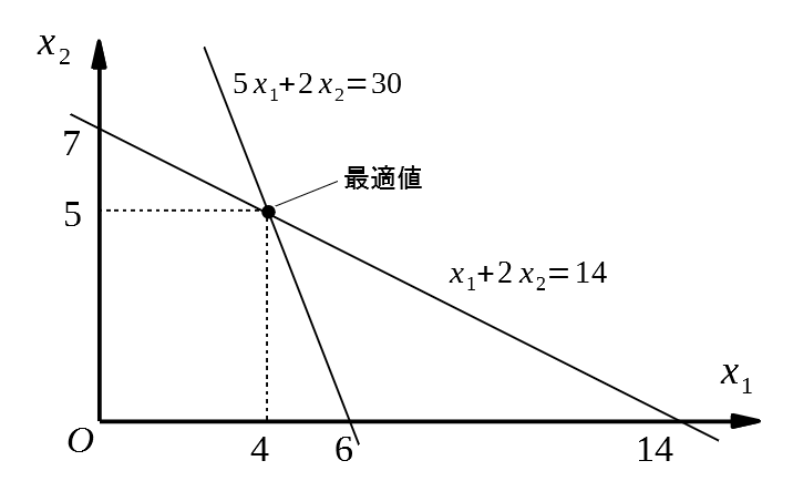
以下の最小化問題を考える。
\( \begin{array}{ll} \text{minimize} & -5x_1-4x_2 \\\ \text{subject to} & 5x_1+2x_2 \le 30 \\\ & x_1 + 2x_2 \le 14 \\\ & x_1 \ge 0, x_2 \ge 0 \end{array} \)
図示すると以下のようになり、\((x_1, x_2)=(4, 5)\)で最小値\( -40\)をとる。
Pyomoのソースコード #
上記の線形計画問題をPyomoを使って記述し、最適化を実行したコードは以下のようになる。
import pyomo.environ as pyo

model = pyo.ConcreteModel(name="LP sample",
                          doc="2 variables, 2 constraints")

model.x1 = pyo.Var(domain=pyo.NonNegativeReals)
model.x2 = pyo.Var(domain=pyo.NonNegativeReals)

model.OBJ = pyo.Objective(expr = -5*model.x1 -4*model.x2,
                          sense = pyo.minimize)

model.Constraint1 = pyo.Constraint(expr = 5*model.x1 + 2*model.x2 <= 30)
model.Constraint2 = pyo.Constraint(expr = model.x1 + 2*model.x2 <= 14)

opt = pyo.SolverFactory('glpk')
res = opt.solve(model)

print(f"評価関数:{model.OBJ()}")
print(f"x1: {model.x1()}")
print(f"x2: {model.x2()}")
実行結果は以下のようになり、最適値を得られている。
評価関数:-40.0
x1: 4.0
x2: 5.0
ソースコードの解説 #
以下、ソースコードの詳細を述べる。
問題のオブジェクトの作成 #
まず、ConcreteModelクラスを用いて問題のオブジェクトを作成する。
model = pyo.ConcreteModel(name="LP sample",
                          doc="2 variables, 2 constraints")
pyomoでは問題を定義するためのクラスには、次の2種類がある。
ConcreteModel: 具体的なパラメータを定義しながら作成するAbstractModel: パラメータは後で設定する
ここではConcreteModelを用いた。
また、name, docという引数では、それぞれモデルの名前と説明を文字列 (str) で設定している。これらの値を取得するには、オブジェクトのname, docメンバ変数を呼ぶ。
例:
>>> model.name
'LP sample'
勿論、name, docは設定する必要はなく、以下のようにしても良い。
model = pyo.ConcreteModel()
変数の定義 #
次に、Varクラスを用いて変数を定義する。
model.x1 = pyo.Var(domain=pyo.NonNegativeReals)
model.x2 = pyo.Var(domain=pyo.NonNegativeReals)
modelにx1, x2といった適当な変数を作り、Varクラスのオブジェクトとする。
Varクラスの引数domainは変数の種類を表す。Pyomoで定義可能なdomainの一部を以下に示す。
RealsPositiveRealsNonPositiveRealsNegativeRealsNonNegativeRealsIntegersPositiveIntegersNonPositiveIntegers
また、Varクラスの引数boundsとinitializeでそれぞれ変数の範囲と初期値を定義できる。
例:
pyo.Var(domain=pyo.NonNegativeReals,
        bounds=(3, 6), initialize=5)
目的関数の定義 #
次に、Objectiveクラスを用いて目的関数を定義する。
model.OBJ = pyo.Objective(expr = -5*model.x1 -4*model.x2,
                          sense = pyo.minimize)
先ほど定義した変数x1, x2を用いて、exprに目的関数を記述する。
また、senseで最小化問題(minimize)か最大化問題(maximize)かを定義する(初期値はminimize)。
目的関数を定義する方法として、以下のように関数を定義してruleに渡す方法もある。
def ObjRule(model):
    return -5*model.x1 -4*model.x2

model.OBJ = pyo.Objective(rule = ObjRule,
                          sense = pyo.minimize)
なお、ConcreteModelではexprとruleのどちらも使えるが、AbstractModelではruleしか使えない。
制約条件の定義 #
Constraintクラスで制約条件を設定する。
model.Constraint1 = pyo.Constraint(expr = 5*model.x1 + 2*model.x2 <= 30)
model.Constraint2 = pyo.Constraint(expr = model.x1 + 2*model.x2 <= 14)
等式制約は==で、不等式制約は<=, >=でそれぞれ設定する。
目的関数と同様に、exprの代わりにruleと関数で制約条件を定義できる。
例:
def ConstRule1(model):
    return 5*model.x1 + 2*model.x2 <= 30

model.Constraint1 = pyo.Constraint(rule = ConstRule1)
ソルバの指定と最適化 #
最後に、ソルバを指定して最適化を行う。
opt = pyo.SolverFactory('glpk')
res = opt.solve(model)
SolverFactoryでソルバを指定し、solveメソッドで最適化を行う。resには最適化の結果が格納される。
また、solveでtee=Trueとすると、ソルバの出力が表示される。
res = opt.solve(model, tee=True)
最適化結果の評価 #
最適化後の変数や目的関数の値を取得するには、modelの変数に直接アクセスする。
>>> model.OBJ()
-40.0
>>> model.x1()
4.0
>>> model.x2()
5.0
最適化問題の概要を表示するには、model.display(), model.pprint()などを実行する。
>>> print(model.display())
Model LP sample

  Variables:
    x1 : Size=1, Index=None
        Key  : Lower : Value : Upper : Fixed : Stale : Domain
        None :     0 :   4.0 :  None : False : False : NonNegativeReals
    x2 : Size=1, Index=None
        Key  : Lower : Value : Upper : Fixed : Stale : Domain
        None :     0 :   5.0 :  None : False : False : NonNegativeReals

  Objectives:
    OBJ : Size=1, Index=None, Active=True
        Key  : Active : Value
        None :   True : -40.0

  Constraints:
    Constraint2 : Size=1
        Key  : Lower : Body : Upper
        None :  None : 14.0 :  14.0
    Constraint1 : Size=1
        Key  : Lower : Body : Upper
        None :  None : 30.0 :  30.0
None
>>> print(model.pprint())
2 variables, 2 constraints

    2 Var Declarations
        x1 : Size=1, Index=None
            Key  : Lower : Value : Upper : Fixed : Stale : Domain
            None :     0 :   4.0 :  None : False : False : NonNegativeReals
        x2 : Size=1, Index=None
            Key  : Lower : Value : Upper : Fixed : Stale : Domain
            None :     0 :   5.0 :  None : False : False : NonNegativeReals

    1 Objective Declarations
        OBJ : Size=1, Index=None, Active=True
            Key  : Active : Sense    : Expression
            None :   True : minimize : -5*x1 - 4*x2

    2 Constraint Declarations
        Constraint1 : Size=1, Index=None, Active=True
            Key  : Lower : Body        : Upper : Active
            None :  -Inf : 5*x1 + 2*x2 :  30.0 :   True
        Constraint2 : Size=1, Index=None, Active=True
            Key  : Lower : Body      : Upper : Active
            None :  -Inf : x1 + 2*x2 :  14.0 :   True

    5 Declarations: x1 x2 OBJ Constraint2 Constraint1
None
ソルバの結果を表示するには、opt.solve()の戻り値をprintで表示する。
>>> print(res)
Problem:
- Name: unknown
  Lower bound: -40.0
  Upper bound: -40.0
  Number of objectives: 1
  Number of constraints: 3
  Number of variables: 3
  Number of nonzeros: 5
  Sense: minimize
Solver:
- Status: ok
  Termination condition: optimal
  Statistics:
    Branch and bound:
      Number of bounded subproblems: 0
      Number of created subproblems: 0
  Error rc: 0
  Time: 0.17183566093444824
Solution:
- number of solutions: 0
  number of solutions displayed: 0
参考 #
Pyomoの公式リファレンス
Pyomo Documentation 5.6.9 — Pyomo 5.6.9 documentation
GLPKについて
GLPK - GNU Project - Free Software Foundation (FSF)
参考にさせていただいた日本語の記事