PyomoとIPOPTで非線形計画問題を解く

はじめに

PyomoはPythonで書かれた最適化モデリングツールである。Pyomoの基本的な使い方と、線形計画問題の解き方については以下の記事を参照。
Pyomoで線形計画問題を解く

本記事では、Pyomoを使って非線形計画問題を解く方法を示す。Pyomoには最適化ソルバが含まれていないため、IPOPT (Interior Point OPTimizer)という無償ソルバーを使う。IPOPTは主双対内点法を利用したソルバであり、大規模な非線形問題を高速に解くことができる。問題は連続である必要がある。また、大域的最適解を求めるには問題が凸である必要がある。

環境は以下の通り。

ソフトウェア	バージョン
Python	3.7.4
Pyomo	5.6.9
IPOPT	3.11.1

ソフトウェアのインストール

PyomoとIPOPTをインストールする。conda環境の場合は以下を実行する。

conda install -c conda-forge pyomo
conda install -c conda-forge ipopt

pip環境の場合は以下を実行する。

pip install pyomo
pip install ipopt

対象とする線形計画問題

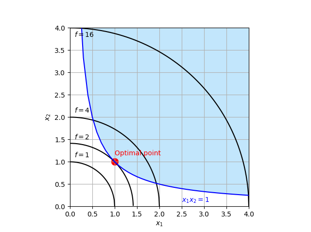
以下の制約付き非線形最小化問題を考える。

$$ \begin{array}{ll} \text{minimize} \ & f(x_1, x_2) = x_1^2 + x_2^2 \\ \text{subject to} \ & x_1 x_2 \ge 1 \\ & x_1 \ge 0, x_2 \ge 0 \end{array} $$

図示すると以下のようになり、$(x_1, x_2)=(1, 1)$で最小値$ 2$をとる。青色で図示した領域は実行可能領域を示す。

pyomo-nlp

Pyomoのソースコード

上記の問題をPyomoを使って記述し、最適化を実行したコードは以下のようになる。

 1
 2
 3
 4
 5
 6
 7
 8
 9
10
11
12
13
14
15
16


import pyomo.environ as pyo

model = pyo.ConcreteModel(name="NLP sample",
                          doc="2 variables, 1 constraints")
model.x = pyo.Var([1,2], domain=pyo.NonNegativeReals) # 変数を定義
model.OBJ = pyo.Objective(expr = model.x[1]**2 + model.x[2]**2,
                          sense = pyo.minimize) # 目的関数を定義
model.Constraint = pyo.Constraint(expr = model.x[1] * model.x[2] >= 1)
# 制約条件を定義

opt = pyo.SolverFactory('ipopt') # 最適化ソルバを設定
res = opt.solve(model) # 最適化計算を実行

print(f"評価関数：{model.OBJ()}")
print(f"x1: {model.x[1]()}")
print(f"x2: {model.x[2]()}")

実行結果は以下のようになり、最適値を得られている。

1
2
3


評価関数：1.9999999825046202
x1: 0.999999995626155
x2: 0.999999995626155

ソースコードの解説

以下、ソースコードの詳細を述べる。

問題のオブジェクトの作成

まず、ConcreteModelクラスを用いて問題のオブジェクトを作成する。

1
2


model = pyo.ConcreteModel(name="NLP sample",
                          doc="2 variables, 1 constraints")

pyomoでは問題を定義するためのクラスには、次の2種類があるが、ここではConcreteModelを用いた。

ConcreteModel: 具体的なパラメータを定義しながら作成する
AbstractModel: パラメータは後で設定する

また、name, docという引数では、それぞれモデルの名前と説明を文字列 (str) で設定している。これらの値を取得するには、オブジェクトのname, docメンバ変数を呼ぶ。

例：

1
2


>>> model.name
'NLP sample'

勿論、ConcreteModelクラスは引数を与える必要はなく、単に以下のようにしても最適化の結果には影響しない。

1

model = pyo.ConcreteModel()

変数の定義

次に、Varクラスを用いて変数を定義する。

1

model.x = pyo.Var([1,2], domain=pyo.NonNegativeReals) # 変数を定義

modelにxといった適当なメンバ変数を作り、Varクラスのオブジェクトを定義する。

Varクラスの第1引数に数値のリストを割り当てることで、xはそのリストと同じ長さのベクトルになる。

また、Varクラスの引数domainは変数の種類を表す。Pyomoで定義可能なdomainの一部を以下に示す。

Reals
PositiveReals
NonPositiveReals
NegativeReals
NonNegativeReals
Integers
PositiveIntegers
NonPositiveIntegers

また、Varクラスの引数boundsとinitializeでそれぞれ変数の範囲と初期値を定義できる。

例：

1
2


pyo.Var([1,2], domain=pyo.NonNegativeReals,
        bounds=(3, 6), initialize=5)

目的関数の定義

次に、Objectiveクラスを用いて、目的関数を定義する。

1
2


model.OBJ = pyo.Objective(expr = model.x[1]**2 + model.x[2]**2,
                          sense = pyo.minimize) # 目的関数を定義

先ほど定義した変数xを用いて、exprに目的関数を記述する。

また、senseで最小化問題(minimize)か最大化問題(maximize)かを定義する（初期値はminimize）。

目的関数を定義する方法として、以下のように関数を定義して、ruleに渡す方法もある。

1
2
3
4
5


def ObjRule(model):
    return model.x[1]**2 + model.x[2]**2

model.OBJ = pyo.Objective(rule = ObjRule,
                          sense = pyo.minimize)

なお、ConcreteModelではexprを使う方法とruleを使う方法のどちらも使えるが、AbstractModelではruleを使う方法しか使えない。

制約条件の定義

Constraintクラスで制約条件を設定する。

1
2


model.Constraint = pyo.Constraint(expr = model.x[1] * model.x[2] >= 1)
# 制約条件を定義

等式制約は==で、不等式制約は<=, >=でそれぞれ設定する。
Objectiveクラスの場合と同様に、exprの代わりに、ruleと関数で制約条件を定義することができる。

例：

1
2
3
4


def ConstRule(model):
    return model.x[1] * model.x[2] >= 1

model.Constraint1 = pyo.Constraint(rule = ConstRule)

ソルバの指定と最適化

最後に、ソルバを指定して最適化を行う。

1
2


opt = pyo.SolverFactory('ipopt')
res = opt.solve(model)

SolverFactoryでソルバを指定する。ここではIPOPTを用いる。次に、SolverFactoryオブジェクトのsolveメソッドにmodelを指定して実行すると、最適化が行われる。resには最適化の結果が格納される。
また、solveでtee=Trueとすると、ソルバの出力が表示される。

1

res = opt.solve(model, tee=True)

最適化ソルバのオプション設定

最適化ソルバ（ここではIPOPT）にオプションを設定するためには、最適化計算の前に、SolverFactoryオブジェクトのoptions変数に辞書形式で渡す。

例：

1
2
3
4
5


opt = pyo.SolverFactory('ipopt')
opt.options = {"print_level" : 4,
               "tol" : 1E-3}

res = opt.solve(model, tee=True)

もしくは、以下のようにしてもよい。

1
2
3
4
5


opt = pyo.SolverFactory('ipopt')
opt.options["print_level"] = 4
opt.options["tol"] = 1E-3

res = opt.solve(model, tee=True)

上記の例では、

最適化計算のログ出力の詳細度合い (print_level) を4（0～12の範囲。数字が大きいほど詳細になる）
最適解の許容誤差 (tol) を1E-3

と設定している。

IPOPTで設定可能なオプションについては、以下のページを参照。
Ipopt: Ipopt Options

一覧の形式で確認したい場合には、以下のページを参照。
https://www.coin-or.org/Bonmin/option_pages/options_list_ipopt.html

最適化結果の評価

最適化後の変数や目的関数の値を取得するには、modelの変数に直接アクセスする。

1
2
3
4
5
6


>>> model.OBJ()
1.9999999825046202
>>> model.x[1]()
0.999999995626155
>>> model.x[2]()
0.999999995626155

最適化問題の概要を表示するには、model.display(), model.pprint()などを実行する。

 1
 2
 3
 4
 5
 6
 7
 8
 9
10
11
12
13
14
15
16
17
18
19


>>> print(model.display())
Model NLP sample

  Variables:
    x : Size=2, Index=x_index
        Key : Lower : Value             : Upper : Fixed : Stale : Domain
          1 :     0 : 0.999999995626155 :  None : False : False : NonNegativeReals
          2 :     0 : 0.999999995626155 :  None : False : False : NonNegativeReals

  Objectives:
    OBJ : Size=1, Index=None, Active=True
        Key  : Active : Value
        None :   True : 1.9999999825046202

  Constraints:
    Constraint1 : Size=1
        Key  : Lower : Body               : Upper
        None :   1.0 : 0.9999999912523101 :  None
None

 1
 2
 3
 4
 5
 6
 7
 8
 9
10
11
12
13
14
15
16
17
18
19
20
21
22
23
24
25


>>> print(model.pprint())
2 variables, 1 constraints

    1 Set Declarations
        x_index : Dim=0, Dimen=1, Size=2, Domain=None, Ordered=False, Bounds=(1, 2)
            [1, 2]

    1 Var Declarations
        x : Size=2, Index=x_index
            Key : Lower : Value             : Upper : Fixed : Stale : Domain
              1 :     0 : 0.999999995626155 :  None : False : False : NonNegativeReals
              2 :     0 : 0.999999995626155 :  None : False : False : NonNegativeReals

    1 Objective Declarations
        OBJ : Size=1, Index=None, Active=True
            Key  : Active : Sense    : Expression
            None :   True : minimize : x[1]**2 + x[2]**2

    1 Constraint Declarations
        Constraint1 : Size=1, Index=None, Active=True
            Key  : Lower : Body      : Upper : Active
            None :   1.0 : x[1]*x[2] :  +Inf :   True

    4 Declarations: x_index x OBJ Constraint1
None

最適化の結果を表示するには、opt.solve()の戻り値をprintで表示する。

 1
 2
 3
 4
 5
 6
 7
 8
 9
10
11
12
13
14
15
16
17
18


>>> print(res)
Problem: 
- Lower bound: -inf
  Upper bound: inf
  Number of objectives: 1
  Number of constraints: 1
  Number of variables: 2
  Sense: unknown
Solver: 
- Status: ok
  Message: Ipopt 3.11.1\x3a Optimal Solution Found
  Termination condition: optimal
  Id: 0
  Error rc: 0
  Time: 0.35607051849365234
Solution: 
- number of solutions: 0
  number of solutions displayed: 0